Time seriesSo far, we have mainly been using surface plots at a specific time instance to analyze the simulation outcome. However, it is also possible to extract a time series for one particular surface element. This can sometimes provide a complementary picture. In the context of the software, this is called a 'recording'.Recordings are versatile, in that they allow to access many different parameters, starting from sun elevation angle over radiation fluxes to temperatures. Since they refer to the thermal state of the simulation, a recording requires to have surface elements defined and to run a full evolution.
Days on MercuryWe've stated before that in the case of slow rotation at timescales comparable with the orbital period, the normal method of extracting solar elevation angles fails, and also that the notion of 'standard days' has no absolute timing. Using recordings, both problems can be overcome, however the drawback is that a recording refers to a surface element and hence limits the accuracy in latitude and longitude to the resolution of the grid.Try the following configuration file:
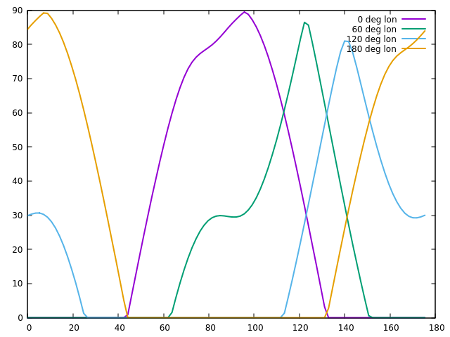
The keyword record initializes the recording procedure. npoints determines the number of points to be plotted (the time resolution of the record is determines from this and the evolution time, and it should go without saying that the thus determined recording timestep cannot be smaller than the evolution timestep). The surface element of the record is identified by index numbers. How do we know it's latitude and longitude? This works via the simulation output, the record is announced with a line Record initialized for element at lat 5.625 and longitude 120. Finally, var_x and var_y denote the variables on the plot axes. Here the x-axis has to be a time variable, but there is a choice between seconds (default), hours, days and years. Running the result for different longitudes reveals the following picture:
Days on Mercury are generally long, and due to the peculiar eccentricity of the orbit the sun moves apparently backward in the sky for a few days. There are longitudes for which this prolongs the duration of the sun in the zenith and locations for which this does not happen - the former correspond to the high-irradiation spots at 0 and 180 degrees longitude.
Analyzing seasonsTime series can be a helpful tool to better analyze several patterns that drive temperature variations. Consider the following, rather complex example of the moon Inferno closely orbiting the hot Jupiter type gas-giant Infernus which in turn orbits a binary star system (never mind questions of stability of orbits or atmospheres at this point, the example is constructed to maximize the effect of indirect radiation and eclipses).Inferno is tidally locked to Infernus, so we expect to see day and night cycles driven by its orbital period, frequent eclipses of both stars by Infernus for the planet-facing hemisphere, as well as binary seasons as the hotter partner moves closer and farther away and infrequent eclipses of the central binary system.
Note the keyword delay_d. We discussed earlier that thermodynamical quantities need some time to reach equilibrium values and be meaningful, and usually we do not want to record this period. A delay period specified with this keyword allows to skip the equilibration part and record only the relevant bits. Running for the planet-facing and opposite hemisphere finds the following:
Generally the planet-facing hemisphere is significantly cooler, and the effect of planetary eclipses during every orbit is clearly seen as a short period of temperature decay - this pattern is absent on the opposite hemisphere which does not experience planetary eclipses. The binary seasons are seen in the slow pattern of decrease/increase of the maximal daily temperatures. Close to day 89, the temperatures drop unusually low - this is the effect of a stellar eclipse in which the cooler Inferno-A covers the hotter Inferno-B. For a system with small axis-tilt, a time series can uncover most of the seasonal variation, however for a more pronounced axis tilt, the interpretation is more difficult and generall both time series and surface plots can be useful to understand the results.
Continue with Atmospheres. Back to main index Back to science Back to worldbuilder Created by Thorsten Renk 2022 - see the disclaimer, privacy statement and contact information. |

