Temperature evolutionThe study of temperatures on a planetary surface is more interesting and relevant than irradiation, but also more complicated. We've already covered the concept of thermal inertia, so to recapitulate: The absorbed radiation energy is stored by heating the surface up to a given depth. In this process, the surface gets warmer and radiates energy in the IR band back into space which depletes the stored energy. If one waits long enough, the surface reaches an equilibrium temperature which is defined by the same amoung of energy being absorbed and radiated.However, in practice one usually can not wait long enough - because the planet rotates, the sun angle changes, and so the amount of absorbed energy changes a lot. Typically that leads to a situation in which during the day the thermal reservoir in the ground is filled with energy and temperatures are below radiative equilibrium whereas at night the energy reservoir is depleted and temperatures are hence above radiative equilibrium. How quickly temperatures follow the available energy depends on a number of factors - the active depth, the heat capacity of the surface material and the rotation period of the planet. If the active depth is small, the heat capacity is small and the rotation slow, radiative equilibrium tends to be more easily reached, if the depth is large, the heat capacity is large and the rotation fast, the planet will generally be far from radiative equilibrium. However, what the active depth is depends also on the rotation period. Energy is transported deeper into the material by diffusion, and the typical length scale of a diffusion process grows with the square root of time, so for a longer rotation period, the active depth is expected to grow somewhat. To make this more user-friendly and, the active depth that is specified in the config file is assumed to refer to a standard 24 h day and is scaled automatically assuming a diffusion process when the rotation period of the planet is different. This should usually work (the exception to be discussed later).
ConvergenceLet's start with a simple example, a fairly earth-like planet on a near-circular orbit around a near-sunlike star.
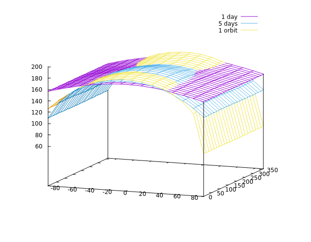
The line var_z temperature instructs the simulation to compute the temperature across the surface after the simulation has been evolved for a day. If you plot this result, it is fairly flat across both latitude and longitude with temperatures ranging from 160-180 K. This isn't so bad since the radiative equilibrium found in the output text is around 173 K. But now let's run the simulation for a full orbital period of 1054.41 days (for this, the keyword evolve_op 1 can also be used) - this should be the same situation, but the temperature profile is different - somewhat higher at the equator, much lower at the poles. How so? Change the time period again to five days and re-run - you should now see this - the temperature is moving towards the situation after one orbit:
This is known as a convergence issue - the simulation is initialized at a given temperature (the radiative equilibrium), but due to the thermal inertia it actually takes time to reach the correct value. So to do a meaningful temperature analysis, you always need to run long enough that the results converge. How to check this? For instance by comparing whether situations which should be near-identical actually are. For instance the situation after two orbits should be, as far as latitude is concerned, the same as after one orbit. If that turns out to be the case, then one orbit simulation before reading off temperatures is enough (in practice usually 30+ days give quite good results already, only very cold surfaces take a long time to cool down).
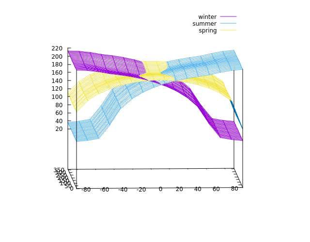
Interpreting temperature plotsIn the absence of an albedo map or complicated spin-orbit resonances, what you see when you project into the latitude axis is seasons, what you see in the longitudinal axis is the daily temperature variation.Let's take a look at seasons first. With an axis tilt of 35 degrees, there should be fairly pronounced seasons. The simulation is, unless otherwise instructed, initialized at periapsis with the axis tilted 90 degrees to the starward direction - which is the northern hemisphere spring equinox. Thus running it for 0.75 orbital periods brings the northern hemisphere winter, to 1.25 periods the northern hemisphere summer.
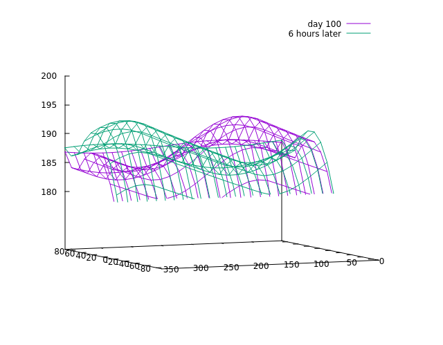
The result shows a planet with strong seasonal temperature variations at the poles, however equatorial temperatures are significantly more stable. Looking along the longitude axis requires a different approach. Let's run the simulation to 100 days and compare with 100.25 days (that is six hours or half a planetary rotation period later) - this shows the following:
There is a high temperature spot that moves around the planet - which is easily interpreted as the part of the planet that is currently in sunlight. For the fast-rotating planet we're looking at, the daily temperature variation is a bit more 10 K. If one changes the rotation period to be longer, say 42 hours, the daily temperature variation grows to a good 20 K. You can experiment with different values for axis tilt or thermal inertia and study the results on daily and seasonal temperature variation.
Continue with Orbital stability. Back to main index Back to science Back to worldbuilder Created by Thorsten Renk 2021 - see the disclaimer, privacy statement and contact information. |


