From random number to texture - GLSL noise functionsA noise function for 3d rendering is a function which inputs at least a coordinate vector (either 2d or 3d) and possibly more control parameters and outputs a value (for the sake of simplicity between 0 and 1) such that the output value is not a simple function of the coordinate vector but contains a good mixture of randomness and smoothness. Dependent on the type of noise, that may mean different things in practice. A noise function is usually chosen based on its ability to represent a natural shape, so it should emulate structures in nature.
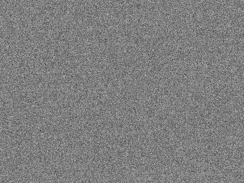
Random numbersAt the core of any noise functions is a (pseudo-)random-number generator, i.e. a function which inputs a coordinate vector and outputs a value between 0 and 1. Unlike the full noise function which is supposed to have smoothness, the raw output of the random number generator may jump wildly even on a short distance and is not supposed to resemble anything.What works well to give an essentially unpredictable output is to use a truncation on a rapidly oscillating function. The following implementations produce viable raw noise for 2d or 3d coordinates:
The result is just a very fine grained surface with pixel to pixel uncorrelated color values between 0 and 1:
Noise function characteristicsThe function above shows what is essentially a pixel to pixel uncorrelated noise - knowing the value of the function at one pixel, one can't say what the value of the adjacent pixel will be. That's not how random patterns in nature typically look. For instance, while the shape of a cloud is not predictable, if one bit of it is opaque white, it's very likely that everything nearby will also be. That is to say, in many natural random patterns there is a correlation length over which the characteristics of the pattern does not change, and only beyond this correlation length the pattern appears random and unpredictable.If one takes a picture of a natural random pattern and runs a Fourier transformation over it, these characteristic length scales would emerge was frequencies (or wavelengths) of the Fourier analysis. In the following, we'll frequently refer to noise 'at a certain wavelength'. The meaning is roughly that the distribution is predictable for any length scale much below that number, but random for any distance above that. This is a statement quite independent of the particular type of noise. Put a different way, noise a 1 m wavelength will create a pattern that looks completely random and point to point uncorrelated when a 10 km x 10 km chunk area is considered, but very homogeneous over a 1 cm x 1 cm patch. Note however that a noise function can have several characteristic wavelengths,
Perlin noisePerlin noise, named after its inventor Ken Perlin, is perhaps the best known example of noise in 3d rendering. It gives a smooth, organic distribution of shapes at a certain wavelength, and by adding noise at different wavelengths, a large variety of effects can be achieved.
Basic ideaThe basic algorithm is surprisingly simple - to generate Perlin noise at a wavelength L:
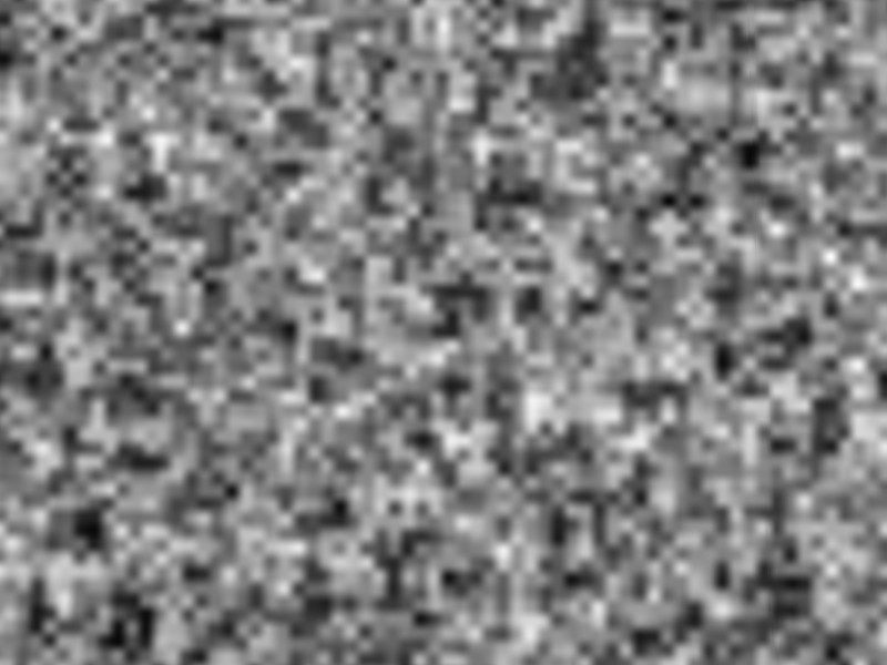
GLSL realizationThe following snippet of code is a 3d variant of Perlin noise, using the smoothstep function to interpolate between grid points.
The raw output of this function, with black representing 0 and white 1, looks like this:
ExamplesA single wavelength of Perlin noise does not look particularly compelling and the beauty of it only emerges after mixing several wavelengths. Often 'octaves' are used in rendering, i.e. Perlin noise is generated for L, L/2, L/4,...L/n and then all are summed with a weight of a constant c to the power of i.Two octaves already look less artificial:
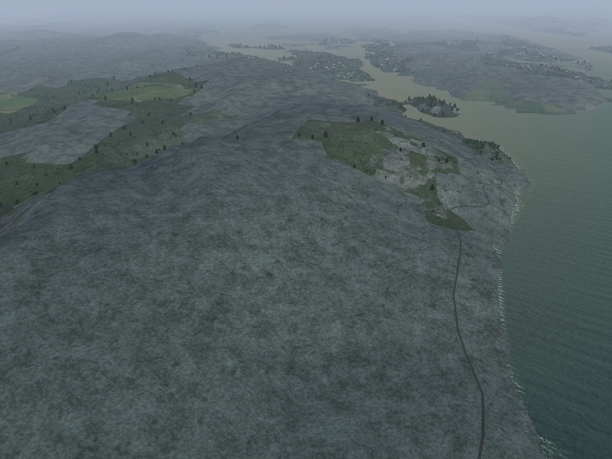
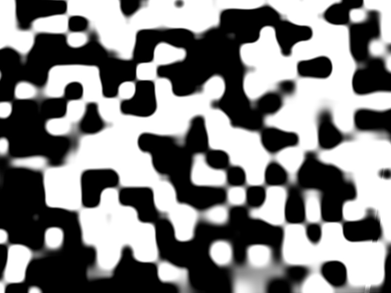
With four octaves added, the result already starts to resemble a rock surface:
Note the regression to the mean - the more octaves are added, the more likely it is to find a value close to 0.5, i.e. to produce a uniform grey surface and any domains where 0 or 1 are reached become rarer and rarer. If that is not the goal, the weight with which octaves are added has to be changed or non-linear post-processing has to be used. If c < 1, then the shorter wavelengths are progressively suppressed and the base pattern is given by long wavelength noise with less visible details determined by finer noise. The following example shows a rock surface generated from Perlin noise with c=0.8 where the base grey color is multiplied with the output of the noise function:
Changing to c=1.3 instead emphasizes the short wavelength noise components and gives visuals which are fairly homogeneous on a large scale but very gritty from close-up:
However, summing Perlin noise in octaves is neither necessary nor always useful. Raw Perlin noise outputs a smooth distribution varying between 0 and 1 with fairly equal probability. Often, a more desirable goal (for instance in blending textures) is to create domains, i.e. regions where the noise function is 0 and other regions where it is 1, separated by a fairly small boundary region in which the values blend into each other. This can nicely be achieved by a non-linear post-processing step, for instance via the smoothstep function as follows:
Here, fraction controls what amount of the area will be zero and what amount unity, and transition how rapid the two domains will blend into each other. Using such a non-linear post-processing, for instance a non-tiling terrain texture can be blended from multiple texture channels:
Sparse dot noiseThe idea underlying sparse dot noise is partially similar to Worley noise, except that it's computationally cheaper because it makes the sparseness assumption. Suppose you have a surface which is covered by comparatively rare, dot-like structures. They're irregularly spaced, but at a mean distance of the noise wavelength. Since they are rare, one can safely assume any two won't overlap.
Basic ideaThe algorithm to generate such a situation is as follows:
GLSL realizationA GLSL realization of the above algorithm is given by the following code which inputs the maximal dot radius and the dot density per cell as additional control parameters:
The raw output of this function, with black representing 0 and white 1, looks like this:
ExamplesThe sparse dot noise algorithm can easily be extended to sometimes place an overlapping dot to a dot, creating a slightly irregular appearance. Also, applying a non-linear filter gives a segmentation into domains. Both techniques can be combined to create for instance the appearance of rain drops on glass procedurally:
Sparse dot actually does not have to be sparse at all. Simply create multiple overlapping grids at slightly different L and draw all the noise patterns on top of each other and you'll get a fairly dense yet still irregular dot distribution. Multiply some of these with a time-dependent periodic function between 0 and 1, and you'll see groups appear and disappear - using enough groups, this is a credible mockup of individual rain drops impacting. The following algorithm is a GLSL realization of this idea (using osg_SimulationTime provided by OpenSceneGraph as the time variable, splash_speed as a measure for how fast the droplets impact and rnorm as the normalized amount of rain). It creates four groups of impact dots from sparse dot noise and fades them in and out in a staggered way controlled by a filtered sine function:
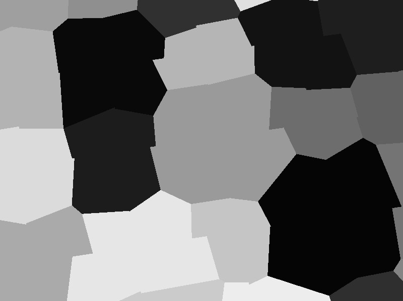
Domain (Voronoi) noiseWe have already mentioned above that it's sometimes useful to have a function which segments a surface into domains which can then be textured separately. If the segmentation is to have an organic look, Perlin noise works fine. However, for man-made structures, often a less organic segmentation pattern is useful. Consider for example patches of managed forest or fields (especially in Europe) - they are usually bounded by straight lines, but they may be rather complex polygons rather than simple squares or rectangles. Voronoi noise is a tool to achieve such a segmentation.Basic ideaThe algorithm to generate such a situation is as follows:
(the last two steps are known as Voronoi partitioning). There is (again) a good degree of sloppiness to this algorithm, in particular a distorted regular grid doesn't give the same amount of randomness than covering a surface with randomly placed points, and limiting the Voronoi partitioning to the four grid points framing the cell also sometimes implies that the wrong domain is assigned. However, in doing so, the algorithm avoids the expensive search over multiple nearest neighbour candidates and performs reasonably fast, while yielding results which look good enough.
GLSL realizationA GLSL realization of the above algorithm is given by the following code which inputs the domain distortion from a regular grid in x and y directions as additional control parameters:
and changes to a more irregular pattern for a high grid distortion:
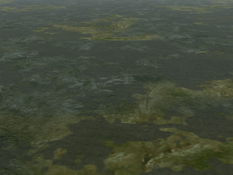
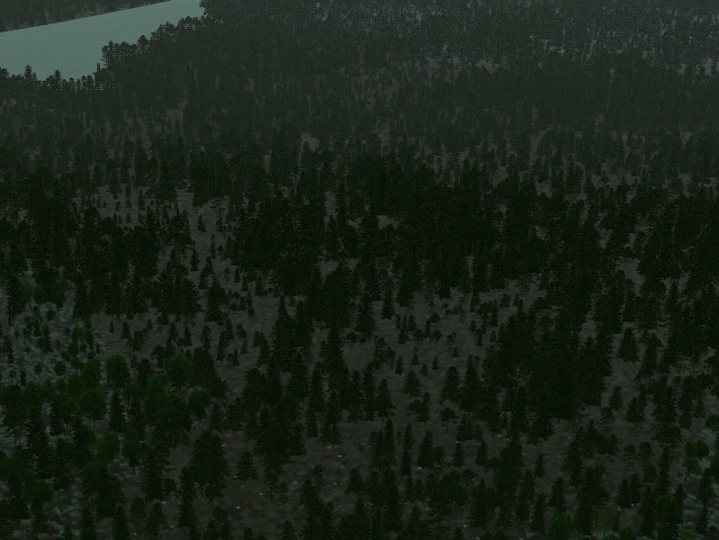
ExamplesUsually one thinks of procedurally generated textures as something to be applied in the fragment shader, but in fact the patterns are often equally useful in the vertex shader to provide regular distortions of geometry. Voronoi noise can for instance be used to quickly get the size distribution of patches in managed forest. Especially in Europe, they tend to be irregular, and often one patch is cut down at a time and then allowed to re-grow for the next fourty years, so a forest always is a collection of domains of trees of different size. Scaling the tree quad size in the vertex shader using Voronoi noise gives a very credible partitioning of that type:
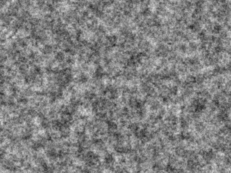
More on non-linear filteringNon-linear filtering as such isn't a technique specific to one noise type, though it has perhaps most applications with Perlin noise. As indicated above, the idea is to map the output of the noise function (which is anywhere between 0 and 1) into the same domain, but non-linearly. For instance, one could map all values below 0.9 to one number and the rest to another number.Such filtering can bring out a surprising number of unexpected shapes out of noise functions. In the following, this is illustrated with Perlin noise of a single wavelength. As a reminder, the noise function itself looks like this:
Filtering this e.g. with
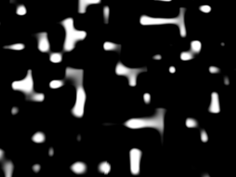
Filtering instead with
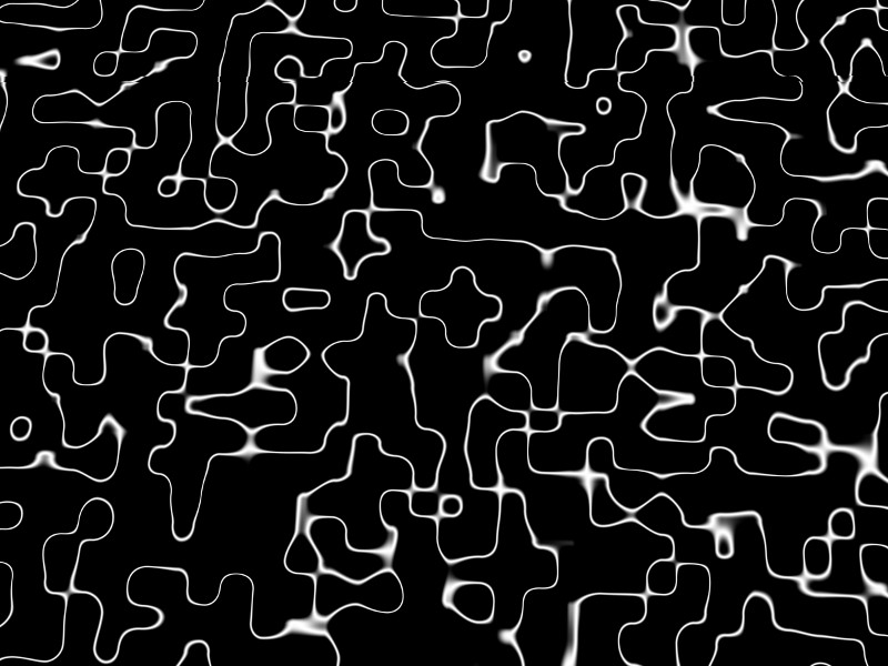
A completely different structure can be obtained by tagging the equipotential lines, i.e. the region where the noise function is close to a given value (here 0.5). Using
Back to main index Back to rendering Created by Thorsten Renk 2015 - see the disclaimer, privacy statement and contact information. |